“A Framework for Variational Inference and Data Assimilation of Soil Biogeochemical Models Using Normalizing Flows”
Grateful and relieved. The two emotions that come to the fore when I try to name my feelings associated with this “uni-batch flow” (as this project was nicknamed by its collaborators) manuscript getting a cross the publication finish line at last following the inception of the project in mid-2020 in the depths of COVID lockdown. Last year at this time, I estimated a 5% chance this manuscript would ever see the light of publication day, so I’ve had a substantial catharsis dump over the past few days from the fact this got out at all. I am also pleased that I was able to accomplish an old frivolous goal to be an author on papers associated with both European Geophysical Union and American Geophysical Union journals.
I am exceedingly grateful to Debora Sujono, whose neat work deriving univariate and multivariate logit-normal random variable distributions for use in the manuscript to supersede use of truncated normal distributions as priors (truncation being critical for biological realism maintenance) and implementations of faster PyTorch NUTS inference benchmarks using Adam Cobb’s hamiltorch package, among other important contributions, were instrumental for carrying the project to the finish line. As a testament to Debora’s dedication and sense of responsibility to this project, she tied up some loose ends and ran some additional experiments referees had requested even as she was preparing to get married and depart from UCI.
Of course, I owe additional hearty thanks to Steve for his rescuing of this paper from the jaws of defeat with sizable cuts and rearrangements in the penultimate stage of review that elevated the progress of the paper from “Major Revisions Needed” to “Accepted with Minor” status. Steve did some heavy lifting in the writing during a time when my bandwidth was exceptionally limited. In an age of LLM-generated LinkedIn-corpo slop, Steve continues to impress with his honed editing and storytelling skills that follow the adage, “You write just enough for the reader to understand, but not enough to understand completely.” (Is that attributed to John McPhee, by the way? Not sure. I read the quote some time ago on Reddit, and haven’t been able to find the originating source since.) Those who know me know I have a tendency to overexplain specifics in my writing in a manner that ends up obfuscating stories, meaning, and intuition.
I mentioned some practical takeaways regarding machine learning model training I sampled from this project in a LinkedIn post. To repeat them separately here, one was the effectiveness of instituting training warmup phases at low learning rates to promote post-warmup training stability and higher peak pre-decay learning rates. Another was the shocking and surprising effectiveness of batch renormalization for reconciling large train-phase and test-phase ELBO gaps. One more takeaway is to always model multivariate, full-rank parameter covariance in variational inference because simplifying mean-field approximation is rarely appropriate and overestimates posterior certainty; even if a data-generating process involved independent distributions for sampling parameter values, it is still appropriate to establish multivariate distribution families to account for potential latent correlations in parameter posteriors revealed through likelihood estimation.
A last takeaway I’ll add is observing firsthand the challenge of comparing inference results and computational speed/efficiency between variational inference (VI) or Markov chain Monte Carlo (MCMC) approaches like the vaunted No-U-Turn Sampler (NUTS). With the differences of VI and MCMC approaches in posteriors (family-constrained versus free to differ nonparametrically from priors), problem framing (optimization versus transition sampling problem), training iteration purposes (ELBO gradient evaluation for backpropagation versus sample accumulation)among other things, it is unfeasible to ensure even start and finish lines for a VI versus MCMC race. Thinking about assessing posterior predictive goodness-of-fit, let alone juxtaposing per-iteration clock speed, yes, we could potentially use a metric like LOO-CV to compare VI and NUTS results, but the comparison may be meaningless due to the lack of start-and-finish alignment. So, comparing Bayesian inference approaches is a hard problem.
What’s also hard? Getting the data needed to perform data inference for parameters of a complex model such as a larger differential equation system with without uncertain-as-hell posteriors. For most applied fields, the state of data products for building inference method and model testbeds still needs work. Compared to where things were at in 2022, there are more greatly welcomed and easily accessible data products available for inference service now.
We had spent a year trying to wrangle together some data from years of Harvard Forest experiments into a suitable data product before it became clear that there were too many gaps to resolve and that development of a Harvard Forest data product for single-site testbed use could likely constitute its own separate project and fell back to exclusive use of synthetic data to fit SCON’s purposes for this manuscript due to time limitations. Fairly, reviewers had held our feet to the fire regarding our lack of empirical data inclusion for more robust demonstration and validation of our normalizing flow approach under real-world data stresses.
So, John Zobitz, Ben Bond-Lamberty, and others are doing critical work for the greater good of soil biogeochemistry. But, unfortunately for poor data assimilation grad students, inference with specific models will remain at least moderately tedious and intensive, as biogeochemical models have a wide array of input requirements and output structures that may require wrangling, processing, extrapolation, augmentation, and/or addition of these once and future data products for model input and output alignment.
For example, if inference is desired for parameters of a soil biogeochemical model that has phosphorous input and a state variable corresponding to phosphorous-associated biomass, but the data product does not include any phosphorous observations, suitable observations will have to be added to and harmonized with the data product. They will likely have to be modeled with great pain and uncertainty. And, if the model state variable units do not match those of the observations, more conversions, modeling, and estimation will be required for model-data integration. For a personal example of that extracted from the unfinished Harvard Forest data product work, soil respiration measurements were observed from square plots of soil and reported as carbon dioxide fluxes per area. However, the models I worked with by default output fluxes per mass unit of carbon. To convert between mass and area, soil depth has to then be accounted for, since it has long been empirically demonstrated that heterotrophic carbon dioxide emissions per volume and mass units of soil greatly varies by soil depth. Hence, for unit alignment, one would either have to (1) map observed data units to model by picking and setting a model corresponding to a certain soil depth layer range (decisions about depth granularity to be made there) and estimating/selecting for some proportion of the area flux assigned to that depth range through a volume to mass via density conversion or (2) go the other way in unit conversions from model to observed data by amalgamating observation outputs from an ensemble of models representing disparate soil depth ranges to correspond to the totality of estimated heterotrophic carbon dioxide flux, transforming from mass to volume to area.
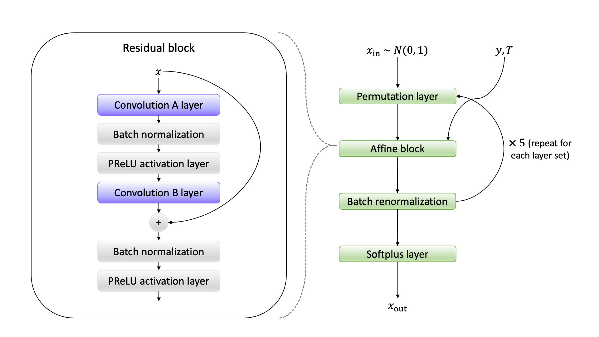
I’ll provide an additional figure bonus in to round out this post. One figure, original Figure 3 in the preprint, was dropped from the final published version of the article, since the figure was confusing reviewers. It was impractical to provide thorough background to introduce all the various machine learning architectures used that have long become known in shorthand in machine learning conference proceedings literature while keeping the manuscript to an acceptable length for a journal, and it made the sense that presenting this figure with limited context ultimately did more to confuse than inform. Because I had missed an obvious error in the process of constructing Panel B of that former figure with TikZ (I had aligned the right “zero pad” label over the wrong array elements), below, I paste both panels of that original figure with a corrected Panel B for posterity:
Original ML architecture ex-Figure 3 Panel A:
Fixed original ML architecture ex-Figure 3 Panel B:

Finally, I wanted to point out that during Wiley’s production process, rendering of the the LaTeX \check symbol a la \(\check{\mu}\) broke so that the symbol no longer aligns directly above characters in the appendix of the published paper:
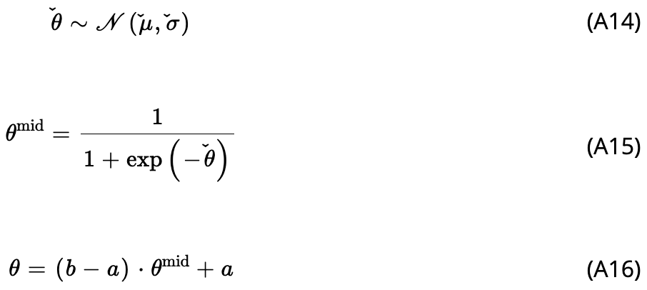
Bummer! The alignment of the logit-normal notation is correct however in the preprint and in this post-revision, pre-publication PDF I’ve uploaded for download.
>> Home